A simple BZ reaction simulation
Background
The Belousov-Zhabotinsky (or “BZ”) reaction is a non-organic chemical reaction known for having a steady-state oscillatory behavior. The initial discovery came from a mixture of chemicals that oscillated in color between yellow and clear. Other forms of the reaction that take place on a surface (such as in a Petri dish) spontaneously evolve moving spiral patterns.
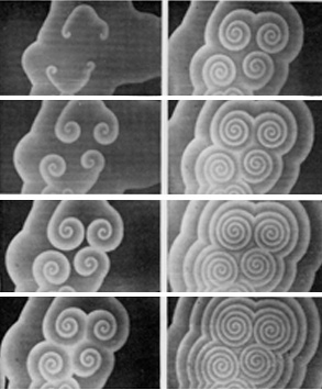
(Image from Zhabotinsky A. M. and Zaikin, A. N., Spatial effects in a self-oscillating chemical system, in Oscillatory processes in biological and chemical systems II, Sel’kov E. E. Ed., Science Publ., Puschino, 1971.)
Many people have tried to characterize this behavior. The FKN model, described by Field, Kőrös, and Noyes in 1971, proposed a set of ten reactions. Two years later, Field and Noyes proposed a simplified five-reaction model called the Oregonator. A paper published in 1990 described 80 distinct reactions that might be involved in the process.
A simple model
Much more recently, Alasdair Turner described a very simple model of the reaction by reasoning from first principles. This model doesn’t attempt to capture the detailed dynamics of the actual chemicals involved in the BZ reaction, but it has the advantage of being extremely simple to reason about. It starts by imagining a set of three reactions:
A + B → 2A (proceeds at rate α)
B + C → 2B (proceeds at rate β)
C + A → 2C (proceeds at rate γ)
Consider the amount of A present at some point in time. The first reaction increases the amount of A based on the amount of B, and the last reaction decreases A based on the amount of C.
Modeling this as a time-step rule would give:
At+1 = At + At * (α * Bt - γ * Ct)
The first At describes the amount present at time t. Most of it will still be present at time t+1. The first reaction produces A at the rate α * At * Bt, due to the Law of mass action. Similarly, the last reaction consumes A at the rate γ * At * Ct. That accounts for all the parts of the time-step rule.
By symmetry, then, there are three rules that describe the three different chemicals:
At+1 = At + At * (α * Bt - γ * Ct)
Bt+1 = Bt + Bt * (β * Ct - α * At)
Ct+1 = Ct + Ct * (γ * At - β * Bt)
The last important bit of this model involves thinking about what happens when these reactions take place on a flat surface, rather than in a well-stirred beaker. Some mixing will take place due to diffusion processes, but that only has local effects. So when figuring the concentration of A in some specific place at time t+1, the values of At, Bt, and Ct should be averaged over some set of neighboring places.
My implementation
Turner’s paper includes a basic implementation of this process in Processing. It follows some basic principles of two-dimensional cellular automata such as Conway’s Game of Life. These systems keep one or more values per pixel, and part of taking a time step involves summing the values in the nine-pixel box around each pixel. Turner’s implementation maintains concentrations of A, B, and C for each pixel, and averages those concentrations when taking a time step. The image that it produces is colored based on all three concentrations, mapping A to red, B to blue, and C to green.
I decided that this would be interesting to play with, so I made a version of my own. My version allows the reaction rates to be controlled dynamically, and it allows reagents to be added and removed from the system. Standard RGB computer graphics limits the number of reagents that can be visually displayed at any point in time to three, but adding more reagents can still show interesting effects.
There are a lot more interesting directions this could be taken in. I haven’t seen any time-step simulation using the Oregonator model, and I’d be curious to see how this one compares. I’d also like to trace the path of several pixels over time, and see if it actually has a chaotic attractor similar to what the original system has. And it would be great to find visually interesting ways of representing concentrations of more than three reagents. But the current thing just seemed worth creating on its own.